Let me start with a good news! Fast Fourier Transform is not another formula. In fact, FFT is not a formula. So, what’s FFT all about? It efficiently crunches the amount of computation required for the Discrete Fourier Transform (DFT) formula we crafted earlier, doing it in a speedy $N\log(N)$ instead of the sluggish $N^2$.

Now, let’s dive into EFFICIENTLY transforming a polynomial from Coefficient Representation to Point-Value representation and we will naturally stumble upon FFT.

Coefficient to Point-Value Representation

Switching from coefficients to points is simple. Take this polynomial:

In coefficient form: 3,2,-4,-1.

To show it in point-value form, we need at least 4 points (for an n degree polynomial, we need n+1). So, let’s choose 1,2,3,4:

• 1 : 3x1 + 2x1 -4x1 -1 = → (1, 0)
• 2 : 3x8 + 2x4 -4x2 -1 = → (2, 23)
• 3 : 3x27 + 2x9 -4x3 -1 = → (3, 86)
• 4 : 3x64 + 2x16 -4x4 -1 = → (4, 207)

For each point, it involves 3 multiplications and 3 additions. In total: 12 multiplications, 12 additions.

note: we also need to calculate the powers of x, but we can re-use the same points for every polynomial, and pre-compute these powers. So I did not account them in here.

The complexity for naive evaluation is roughly d^2, where d is the degree of the polynomial.

That’s not fast, we will try to improve this.

Even and Odd functions

We can be smarter by picking numbers strategically based on the concept of even and odd functions.

• Even functions: symmetry about the y-axis.
• Odd functions: symmetry about the origin.

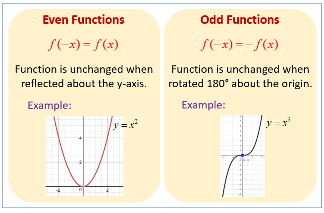
Take an even polynomial:

• 1: Evaluate → (1, 1)
• 2: Evaluate → (2, 4)
• -1: Evaluate → (-1, 1)
• -2: Evaluate → (-2, 4)

For even functions, $f(-x) = f(x)$, letting us evaluate more points without extra work.

For odd functions, $f(-x) = -f(x)$, offering the same efficiency.

To handle any polynomial, we split it into even and odd parts:

Combining E(x) and O(x) brings back our original P(x)! And this comes with some neat properties:

To sum it up: Instead of crunching numbers for 4 points (1,2,3,4) as we did before, now we can simply evaluate our Even and Odd polynomials for 2 points (1, 2).

And then calculate P(x) as follows:

A quick warning:

• Initially, we had 4 equations (evaluating 1,2,3,4 for P(x)).
• Now, we’re still dealing with 4 equations (evaluating 1,2 for E(x) and O(x)).
• However, evaluating P(x) is double the complexity of evaluating E(x) and O(x), thanks to its double degree. Hence, more operations.
• In the end, we’re doing half the work (half the operations) with this new approach.

Our complexity now is: $(N/2)N = N^2 / 2$

It is 2 times better, but in the end, it is still N^2.

We can do even better.

OUTCOME: by using positive-negative symmetry, we can halve the required evaluations.

Divide and Conquer

Right now, we can reduce the amount of points needed to evaluate the polynomial by half. Unfortunately, this reduction can only be applied once. How great would it be if we could employ the same approach for our even and odd functions?

Let’s revisit the example:

But we cannot further divide $E(x)$ into its own even and odd parts because the terms inside $E(x)$ are all even. The same story for $O(x)$… We have to find another way.

Another way

If you think about it, we actually don’t care about the terms being even and odd. We care about positive-negative symmetry. That is why the even and odd functions were useful for us in the first place.

With this mindset, let’s inspect the signs of $1 + x + x^2 + x^3 + x^4 + x^5 + x^6 + x^7$:

• + + + + + + + + for positive $x$.
• + - + - + - + - for negative $x$.

Current situation:

• $E(x)$ + + + + (for negative $x$ values)
• $O(x)$ - - - - (for negative $x$ values)

What we are searching for is, creating the same pattern + - + - for both $E(x)$ and $O(x)$. Then we will be able to further divide $E(x)$ and $O(x)$ to their components by taking advantage of the positive-negative symmetry.

Brainstorming

Let’s think outside of the box. Right now, we are free to create non-sense by pure imagination. Assume that, somehow, we have these signs for

$1 + x + x^2 + x^3 + x^4 + x^5 + x^6 + x^7$:

• + + + + + + + + (for positive $x$ values)
• + + - - + + - - (for ?)

Then, we have:

• + + + + for $E(x)$ (for positive $x$ values)
• + - + - for $E(x)$ (for ?)
• + + + + for $O(x)$ (for positive $x$ values)
• + - + - for $O(x)$ (for ?)

Wohoo! In an imaginary world, we solved our previous problem. We can further divide $E(x)$ and $O(x)$ to their positive and negative parts (as we previously split $P(x)$ into its own even(positive) and odd(negative) parts).

We just need to find the ? (if such a value exists in the first place).

Finding ?

Thinking outside of the box is not easy. One good approach is to focus on what we already know and deduce more abstract generalizations from it.

Again, I present you: $1 + x + x^2 + x^3 + x^4 + x^5 + x^6 + x^7$:

Any negative $x$ value will produce the below signs, right?

+ - + - + - + -

Why so? Why do negative numbers create such a pattern?

The above questions might sound stupid, and you might be rolling your eyes. But to find the essence of knowledge, we sometimes need to ask such questions.

To have the pattern + - + - + - + -, we need to flip the sign each time when we multiply with $x$, right? Each time we increment the power of $x$, we want the sign to flip.

And that’s why any negative number would do for our needs.

Let’s try to apply the same steps to the pattern:

+ + - - + + - -

We need to flip the sign each time when we multiply with $x^2$, right? And flipping the bit means, basically multiplying with $-1$. Each time we increment the power of $x$ by 2, we want the sign to flip.

So, we need to solve this equation:

And the solution to ? in our imaginary world, is an imaginary number, i!

See how those StUPid questions helped us? I hope your attitude towards such basic questions has changed now.

We now have 2 different pairs with 1:

• 1 and -1
• 1 and i

To eliminate potential confusion in the future, we should be able to distinguish them.

• 1 and -1 are pairs, if we want the sign to flip each time we increment the power of $x$, by 1.
• 1 and i are pairs, if we want the sign to flip each time we increment the power of $x$ by 2.

So, let’s say:

• 1 and -1 are pairs in $x^1$ space.
• 1 and i are pairs in $x^2$ space.

Using i as a root to create symmetry

Coming back to where we left off:

Now we can divide $E(x)$ into its own even and odd parts. I know even and odd does not make sense. Think of them as more even and more odd if you will! Let me demonstrate on $E(x)$:

• $$E(1) = 2 - 1$$
• $$E(i) = -2 - 1$$

So, we have:

where:

• $$EE(x) = -1$$
• $$EO(x) = 2x^2$$

$EE(x)$ is a constant function (the input $x$ does not have any effect on it). So, we can say $EE(x) = EE(y)$.

As previously, the odd part $EO(x)$ will flip the sign between inputs. However, instead of the pair 1 and -1, we have 1 and i as a pair for $EO(x)$.

So, instead of evaluating $EO(x)$ for both $1$ and $i$, we can just evaluate it for $1$, and we can let the positive-negative symmetry do the rest of the job for us.

See it yourself: $EO(1) = -EO(i)$.

And $EE(1) = EE(i)$ (remember, constant function).

Note: -i and -1 are also forming a pair in $x^2$ space, just as 1 and i.

OUTCOME: by utilizing i, we can create positive-negative symmetry in $x^2$ space.

Odd functions

Let’s continue with: $O(x) = 3x^3 - 4x \newline = OE(x) + OO(x)$:

• $$OE(x) = -4x$$
• $$OO(x) = 3x^3$$

For $OE(x)$, we cannot use our calculation for $OE(1)$ to derive $OE(i)$. You see why? Because the power of $x$ is only 1. And we need $x^2$ in order to make 1 and i a positive-negative pair. This is a problem… Our optimization is hindered.

For $OO(x)$, can we use our calculation for $OO(1)$ to derive $OO(i)$? Well, yes and no. $3x^3$ includes $x^2$ but there is a remainder $x$.

Check it yourself, we cannot say $OO(1) = -OO(i)$.

Damn, it worked great with the Even variant…

Manipulating Odd variant

Oh yes! That’s the solution: it worked great with the Even variant.

If we somehow make Odd variants look like the Even variants, our problems should be solved.

Let’s redefine the Odd variants by factoring an $x$ out of them, hence, making the powers of $x$ even.

And for the next level:

• $$E(x) = EE(x) + x^2EO(x)$$
• $$O(x) = OE(x) + x^2OO(x)$$

Notice that each recursion, we increment the power of $x$ that we will factor out.

In this case:

• EE(x) = -1
• EO(x) = 2
• OE(x) = -4
• OO(x) = 3

Good news! Now all of them are constant functions, which means, we can rewrite them like this:

• EE = -1
• EO = 2
• OE = -4
• OO = 3

OUTCOME: by factoring out the powers of $x$ from odd functions (w.r.t the recursion level), we achieve consistency across steps, which is crucial for creating an algorithm.

Big Picture Reminder

Let me remind you the big picture.

We initially needed 4 points to evaluate $P(x)$. Then we used even and odd functions, requiring only 2 points for evaluation (the other 2 points will require no computation to be evaluated).

Now, we don’t even need 2 points; we can reduce them to 1 point, with the other point derived without any computation. In fact, we can evaluate ALL possible polynomials (no matter the degree) with a single point with this approach!

Let’s do some examples to make everything crystal clear.

An Example Run

Our polynomial is:

For each approach, we need to evaluate $P(x)$ for 4 points: $x_1$, $x_2$, $x_3$, and $x_4$.

1st approach (naive):

In this approach, we can plug any 4 points into $P(x)$, resulting in $(n+1)(n)$ multiplications and $(n+1)(n-1)$ additions.

Possible points to evaluate:

• $$x_1 = 1$$
• $$x_2 = 2$$
• $$x_3 = 3$$
• $$x_4 = 4$$

This is not efficient…

We went over that already. No need to recompute all the values for $1,2,3,4$ for $P(x)$. Let’s proceed to the next approach.

2nd approach (Even and Odd):

Remembering our polynomial: $P(x) = 3x^3 + 2x^2 -4x -1$

We will leverage Even and Odd functions to duplicate computation across positive-negative pairs, doing only half of the computation.

We cannot use the previous points: 1,2,3,4 for this approach, because we need negative-positive pairs:

• $x_1$ = 1
• $x_2$ = -1
• $x_3$ = 2
• $x_4$ = -2

Recall: computing $E(x)$ gives us the evaluation for $E(-x)$, and the same goes for $O(x)$. Plug $1,2$ into $E(x)$ and $O(x)$, and derive the evaluations for $-1$ and $-2$ without computation.

Denoting even and odd functions for $P(x)$, and summarizing optimizations:

Plugging our 4 points:

• $$x_1 = 1$$
• $$x_2 = -1$$
• $$x_3 = 2$$
• $$x_4 = -2$$

We get:

• $$P(x_1) = E(x_1) + xO(x_1)$$
• $$P(x_2) = E(x_2) - xO(x_2)$$
• $$P(x_3) = E(x_3) + xO(x_3)$$
• $$P(x_4) = E(x_4) - xO(x_4)$$

Considering $x_1$ and $x_2$ are positive-negative pairs, and the same goes for $x_3$ and $x_4$, we can now take advantage of the optimization:

• $$P(x_1) = E(x_1) + xO(x_1)$$
• $$P(x_2) = E(x_1) - xO(x_1)$$
• $$P(x_3) = E(x_3) + xO(x_3)$$
• $$P(x_4) = E(x_3) - xO(x_3)$$

So, we only compute $E(x_1)$, $E(x_3)$, $O(x_1)$, and $O(x_3)$. No need to compute $E(x_2)$, $E(x_4)$, $O(x_2)$, and $O(x_4)$. This saves us half the computations!

3rd approach (Divide and Conquer)

One might call this approach recursive even and odd.

Remembering our polynomial: $P(x) = 3x^3 + 2x^2 -4x -1$

We cannot use the previous points: 1,-1,2,-2 for this approach, because we need negative-positive pairs also in $x^2$ space:

• $x_1$ = 1
• $x_2$ = -1
• $x_3$ = i
• $x_4$ = -i

We have: $P(x) = E(x) + xO(x)$

We have to evaluate $P(x)$ for 4 points:

• $$P(x_1) = E(x_1) + xO(x_1)$$
• $$P(x_2) = E(x_2) + xO(x_2)$$
• $$P(x_3) = E(x_3) + xO(x_3)$$
• $$P(x_4) = E(x_4) + xO(x_4)$$

Considering $x_1$ and $x_2$ are positive-negative pairs (in $x^1$ space), and the same goes for $x_3$ and $x_4$, we can now take advantage of the optimization:

• $$P(x_1) = E(x_1) + xO(x_1)$$
• $$P(x_2) = E(x_1) - xO(x_1)$$
• $$P(x_3) = E(x_3) + xO(x_3)$$
• $$P(x_4) = E(x_3) - xO(x_3)$$

So, we only compute $E(x_1)$, $E(x_3)$, $O(x_1)$, and $O(x_3)$. No need to compute $E(x_2)$, $E(x_4)$, $O(x_2)$, and $O(x_4)$, saving us half the computations!

Since:

Where:

• $$EE(x) = -1$$
• $$EO(x) = 2$$
• $$OE(x) = -4$$
• $$OO(x) = 3$$

We can expand our equations to this:

• $$P(x_1) = EE + x_1^2EO + x_1(OE + x_1^2OO)$$
• $$P(x_2) = EE + x_1^2EO - x_1(OE + x_1^2OO)$$
• $$P(x_3) = EE + x_3^2EO + x_3(OE + x_3^2OO)$$
• $$P(x_4) = EE + x_3^2EO - x_3(OE + x_3^2OO)$$

Considering $x_1$ and $x_3$ are positive-negative pairs (in $x^2$ space), we can now take advantage of an additional optimization (replace every $x_3^2$ with $x_1^2$):

So, let’s replace $x_3$ with $x_1$ for those:

• $$P(x_1) = EE + x_1^2EO + x_1(OE + x_1^2OO)$$
• $$P(x_2) = EE + x_1^2EO - x_1(OE + x_1^2OO)$$
• $$P(x_3) = EE + x_1^2EO + x_3(OE + x_1^2OO)$$
• $$P(x_4) = EE + x_1^2EO - x_3(OE + x_1^2OO)$$

We should compute only $x_1^2EO$ and $x_1^2OO$. No need to compute $x_3^2EO$ and $x_3^2OO$.

Generalizing the solution: Roots of Unity

You might have noticed that: 1,-1,i,-i, these are all solutions to the 4th root of 1. And this is no coincidence. We needed 4 points, and the most clever points to choose from, were the the 4th roots of 1.

If we are to generalize this, by using the roots of 1, we can have 2, 4, 8, 16, … as many roots as we like. And these roots will satisfy the properties we require.

These points (roots) do have a special name: Roots of Unity. These are just equally spaced points on the unit circle.

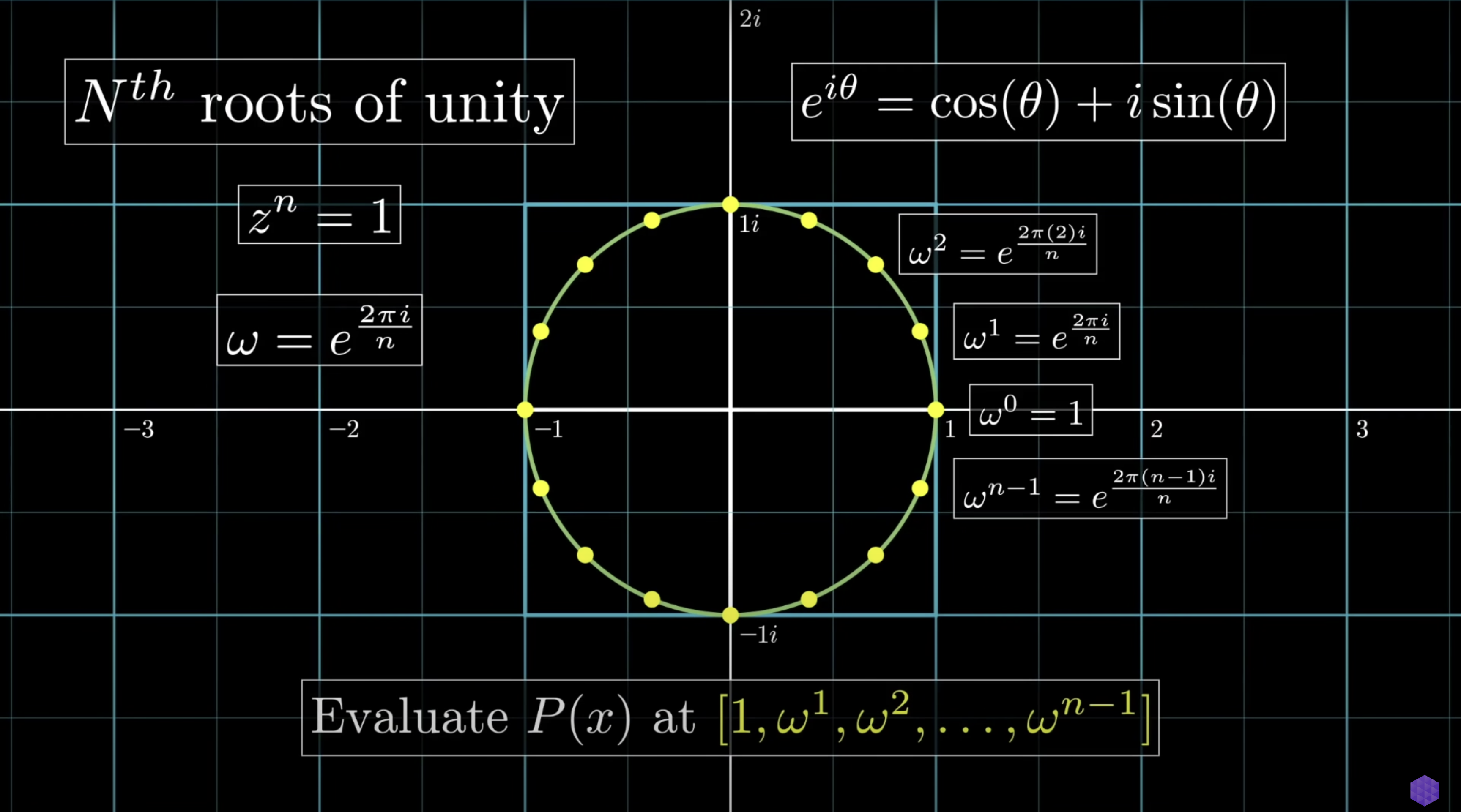
Powers of i, -i, -1, and 1 are periodic, fitting the circular nature. Their powers repeat as they move along the edge of the circle, creating periodicity.

Who would have thought that circles and periods could assist us in evaluating polynomials!

Look at our root of unity formula:

Looks familiar, doesn’t it?

Now, let’s recall our DFT formula for polynomials (the same as waves but with changed letters for clarity):

And recall:

Replace x:

See the resemblance? It is the same formula!

That’s it! This is how we efficiently transform from coefficient form to point-value form. For the reverse direction, apply the inverse DFT (which we discovered).

Here is a video with an FFT example. I’ll provide one myself below with more explanations.

Wrapping Everything Back Together

Our formula is equal to:

• When we plug x into the polynomial A, the result equals the right side (the evaluation of the polynomial A at point x)
• So, our DFT formula is actually evaluating our polynomial at some given point x.

To compute this formula more efficiently, we pick roots of unity for the x values (as given below):

Now, for a degree 3 polynomial, we pick the smallest power of 2 greater than 3:

This equation tells us we need at least 4 points. So, we will do 4 evaluations (for each root of unity) for each root of unity:

Noticing the Efficiency

Remembering our polynomial: $P(x) = 3x^3 + 2x^2 -4x -1$

We can now evaluate our polynomial at 4 different roots of unity:

As you can see, we actually only need to compute the following:

• EE + EO = -1 + 2 = 1
• EE - EO = -1 -2 = -3
• OE + OO = -4 + 3 = -1
• OE - OO = -4 -3 = -7

And plugging them back in:

The Code

Here is the python code for FFT for the curious audience (feel free to skip this if you don’t like codes):

import numpy as np
from typing import List, Tuple

def FFT(P:List):
	# P - [p_0, p_1, ... , p_(n-1)] coeff representation
	n = len(P)
	if n == 1:
		return P
	w = np.exp(-2j * np.pi / n) # roots of unity
	P_e, P_o = even(P), odd(P)
	f_e, f_o = FFT(P_e), FFT(P_o)
	y = [0] * n
	n //= 2

	for i in range(n):
		p = pow(w,i)*f_o[i]
		y[i], y[i+n] = f_e[i] + p, f_e[i] - p

	return y

def even(p:List)->List:
	return p[::2]

# n > 1 for sure
def odd(p:List)->List:
	return p[1::2]

Explanation of The Code

This code should make a lot of sense. Let me show:

P_e, P_o = even(P), odd(P)
f_e, f_o = FFT(P_e), FFT(P_o)

• We are dividing what we have into even and odd parts.
• And recursively apply the same strategy we derived to subsequent parts.

p = pow(w,i)*f_o[i]
y[i], y[i+n] = f_e[i] + p, f_e[i] - p

Recall how we represented $P(x)$ and $P(-x)$?

• $$P(x) = E(x) + xO(x)$$
• $$P(x) = E(x) - xO(x)$$

For $E(x)$ and $E(-x)$ we had to go 1 level deeper, and had to use $x^2$

• $$E(x) = EE + x^2EO$$
• $$E(x) = EE - x^2EO$$

The above code is doing exactly that with the relevant roots of unity raised to its power.

A Question

A good question that you can ask to yourself is: Will it work if we use 2, -2, 2i, -2i instead of 1, -1, i, -i?

And the answer is: yes, but with a twist.

You probably remember our last step:

• $$P(x_1) = EE + x_1^2EO + x_1(OE + x_1^2OO)$$
• $$P(x_2) = EE + x_1^2EO - x_1(OE + x_1^2OO)$$
• $$P(x_3) = EE + x_1^2EO + x_3(OE + x_1^2OO)$$
• $$P(x_4) = EE + x_1^2EO - x_3(OE + x_1^2OO)$$

With 2, -1, i, -i:

For 1, -1, i, -i, it is very easy.

• $$P(1) = EE + 1^2EO + 1(OE + 1^2OO)$$
• $$P(-1) = EE + 1^2EO - 1(OE + 1^2OO)$$
• $$P(i) = EE + 1^2EO + i(OE + 1^2OO)$$
• $$P(-i) = EE + 1^2EO - i(OE + 1^2OO)$$

And all we needed to do was compute the below:

• EE + EO
• EE - EO
• OE + OO
• OE - OO

With 2, -2, 2i, -2i:

• $$P(2) = EE + 2^2EO + 2(OE + 2^2OO)$$
• $$P(-2) = EE + 2^2EO - 2(OE + 2^2OO)$$
• $$P(2i) = EE + 2^2EO + 2i(OE + 2^2OO)$$
• $$P(-2i) = EE + 2^2EO - 2i(OE + 2^2OO)$$

And this will work too! However, why on earth would we prefer extra calculations?

This would add an extra step to the code as well. We will have to compute the powers of 2, and multiply each coefficient with the relevant power of 2 in advance before applying the same algorithm to evaluate the polynomial.

What’s next?

That’s really it for the FFT! Congratulations, you probably possess better understanding of FFT than everyone else who haven’t read this post. And I’m not exaggerating. It took me months to come up with all these simplified intuitions.

Yes, you could have looked at some formulas, expand them, and solve some practice problems with pen&paper, but that would only explain HOW it works, not WHY it works. And according to what I’ve seen on internet till now (2024), most people only know the HOW part.

If you want to learn more, in the next post I’ll explain NTT (Number Theoretic Transform), which is same as FFT, but optimized for computers.