What is NTT (Number Theoretic Transform)?

NTT is just FFT, optimized for computers.

In cryptography, using e, i, and π can be tricky for computers because they deal with finite numbers, and using these constants might lead to precision problems and errors.

As a solution, we have a different notion for roots of unity in finite fields (modular arithmetic).

For example, in the finite field modulo 13:

5^4 \equiv 1 \pmod{13} \newline 12^4 \equiv 1 \pmod{13} \newline 8^4 \equiv 1 \pmod{13}\newline 1^4 \equiv 1 \pmod{13} \newline

You can observe that 5, 12, 8, 1 roughly correspond to i, -1, -i, 1 in modulo 13. Similarly:

5^2 \equiv -1 \pmod{13} \newline 12^2 \equiv 1 \pmod{13} \newline 8^2 \equiv -1 \pmod{13}\newline 1^2 \equiv 1 \pmod{13} \newline

Finding Roots of Unity in Finite Fields

We prefer working with prime numbers in cryptography because they offer favorable properties.

In the context of modular arithmetic, when we use the modulo operation (e.g., mod 13), we are essentially operating within finite fields. Here, our finite field size is 13.

We denote the size of our finite field as q, where q is a prime number.
Our goal is to find n roots of unity for this finite field of size q.

If n divides q-1, then there are indeed n roots of unity in this setting.

In the provided example, where n=4 and q=13, we can find 4 roots of unity.

To obtain an n-th root of unity, we select a random non-zero element in the field [1,q). We then apply the formula below:

(x^{(q-1)/n}) \pmod{q}

This process yields one of the four roots of unity, as demonstrated below:

1^3 \equiv 1 \pmod{13} \newline 2^3 \equiv 8 \pmod{13} \newline 3^3 \equiv 1 \pmod{13}\newline 4^3 \equiv 12 \pmod{13} \newline 5^3 \equiv 8 \pmod{13} \newline 6^3 \equiv 8 \pmod{13} \newline 7^3 \equiv 5 \pmod{13}\newline 8^3 \equiv 5 \pmod{13} \newline 9^3 \equiv 1 \pmod{13} \newline 10^3 \equiv 12 \pmod{13} \newline 11^3 \equiv 5 \pmod{13}\newline 12^3 \equiv 12 \pmod{13}

Taking powers of 5 and 8 allows you to obtain 1 and 12. However, the reverse is not true. This distinction leads us to refer to 5 and 8 as primitive n-th roots of unity.

We are particularly interested in primitive n-th roots of unity because they enable us to derive all the other roots of unity. Thankfully, there is a method for finding primitive n-th roots of unity.

(x^{(q-1)/n})^{n/2} \not\equiv 1 \mod q

If a randomly selected x satisfies the above formula, it is indeed a primitive n-th root of unity.

Adapting FFT to NTT?

A(\omega) = \sum_{n=0}^{N-1}a_n\omega^n

Instead of x, we use roots of unity. That’s it. No more e, no more i, no more π.

In summary, to transition from FFT to NTT, we simply replace:

x = e^{-ik2\pi/N}

with:

x = \omega

and pre-compute these roots (omegas) for our setting so that we can supply the roots to our function.

Visually Exploring the FFT (Butterfly)

Let’s go back to FFT for a bit.

The operations we perform to compute FFT are sometimes also referred as butterfly. It will make more sense with images.

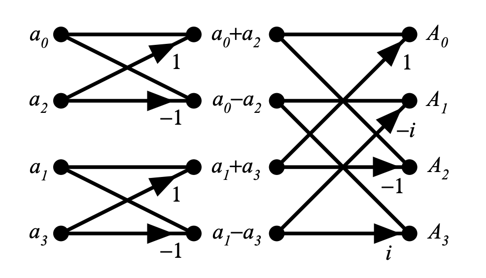image taken from

In the above image, $a_0, a_1, a_2, a_3$ represents the coefficients of a 3rd degree polynomial.

We multiply them with 1 and -1 in the first level,
and with 1, i, -1, and -i in the second level. Take your time and inspect it, it will make a lot of sense.

Here is a demonstration of a 7th degree polynomial that requires 8 evaluations (for 8 different points).

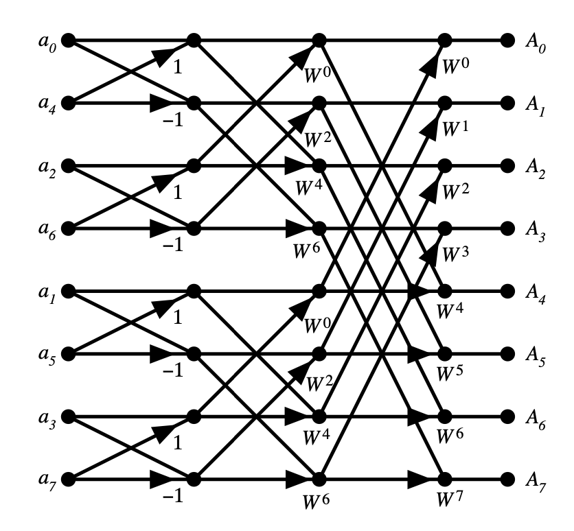image taken from

This time we have 3 levels:

multiply with 1 and -1.
multiply with 1, i, -1, -i.
multiply with w1, w2, w3, w4, w5, w6, w7, and w8 (where you take the 8th power of $w_i$ , you get 1).

Note: replace the imaginary roots with roots in finite field as we described above, and you get NTT. These diagrams won’t change at all for NTT except the roots we multiply with.

The butterfly comes from this:

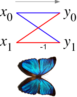
I honestly think it looks more like an hourglass than a butterfly, but ok…

Iterative Approach instead of Recursive

For FFT, our algorithm was recursive (calling itself recursively).

If we use the above images to explain, we start from the left side (but not do the computations), and reach to the right side. Then, we do the calculations from the most far right side, and use what we have computed from right side to find the values on the left side.

If we want to squeeze out the performance, it usually is a good idea to turn recursion into iteration.

Indices of coefficients

I’m going to quote from Paul Heckbert here:

Quote starts…

In the diagram of the 8-point FFT above, note that the inputs aren’t in normal order: $a_0,a_1,a_2,a_3,a_4,a_5,a_6,a_7$ they’re in the bizarre order: $a_0,a_4,a_2,a_6,a_1,a_5,a_3,a_7$ . Why this sequence?

Below is a table of $j$ and the index of the $j$ th input samle, $n_j$ :

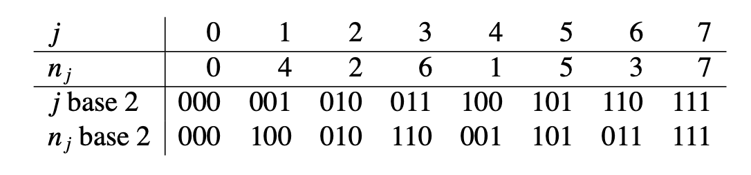
The pattern is obvious if $j$ and $n_j$ are written in binary (last two rows of the table). Observe that each $n_j$ is the bit-reversal of $j$ . The sequence is also related to breadth-first traversal of a binary tree.

Quote ends…

So, we will just reverse the bits for our coefficients indices. That should make the access more straight-forward.

The Code

For those interested, the final version of NTT will look something like this, with some additional optimizations:

import math

def reverse_bits(number, bit_length):
    # Reverses the bits of `number` up to `bit_length`.
    reversed = 0
    for i in range(0, bit_length):
        if (number >> i) & 1:
            reversed |= 1 << (bit_length - 1 - i)
    return reversed

def cooley_tukey_ntt(a, q, omegas):
    n = len(a)
    out = a

    for i in range(n):
        rev_i = reverse_bits(i, n.bit_length() - 1)
        if rev_i > i:
            # swap(out[i], out[rev_i])
            out[i] ^= out[rev_i]
            out[rev_i] ^= out[i]
            out[i] ^= out[rev_i]

    log2n = math.log2(n)

    iterations = int(log2n)
    # below is complicated, but it is actually just to
    # achieve indices of coefficients and roots of unity
    M = 2
    for _ in range(iterations): # recursion into log2n level iterations
        for i in range(0, n, M): # represents the indices of even numbers
            g = 0 # necessary for accessing pre-computed roots of unity
            for j in range(0, M >> 1): # shift needed for finding the next even number
                k = i + j + (M >> 1) # index of odd,
                # where `i` is the index of the even,
                # `j` is the shift that will lead us to next even number
                # and `M` is the gap between `even` and `odd` pair

                U = out[i + j] # even
                V = out[k] * omegas[g] # x * O(x)
                out[i + j] = (U + V) % q # E(x) + xO(x)
                out[k] = (U - V) % q # E(x) - xO(x)
                g = g + n // M # index for finding the next root of unity
        M <<= 1 # double the gap between pairs after each recursion level

    return out

If you prefer the version without comments, the code is available here.

Additionally, you can explore my research paper, where we accelerated the state-of-the-art SEAL library (homomorphic encryption) by 100x through GPU-optimized NTT code:

Thank you for reading!

VI. NTT